Use cases

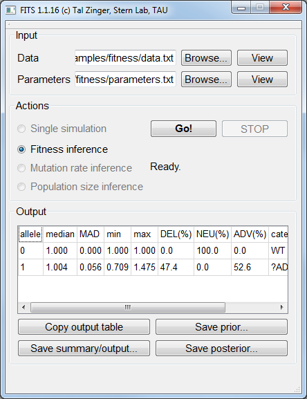
Fitness inference

In Evolve & Resequence (E&R) studies, a population is grown for a period of time under a given condition and sampled at several time points. The frequencies of genetic variants or phenotypes for the different time points are measured, and we’d like to infer the fitness that is associated with each specific variant (or phenotype). An example for such frequency data, sampled for 15 generations and determined for frequency is described here:

The size of the population is estimated to be 100,000. Therefore the parameter N 100000 was set.

The mutation rate is estimated to 1:100,000 (or 10^-5). Therefore the parameter mutation_rate0_1 1e-05 was set.

We expect the fitness values of the phenomena to be between 0 (the minimum possible fitness value) and 2 (very adaptive fitness). Therefore the parameter min_fitness_allele1 0.0 was set, to indicate zero minimal expected fitness and max_fitness_allele1 2.0 as well, to indicate the maximal possible fitness value of two.

The prior we chose for this analysis was smoothed_composite, a prior that is built towards typical fitness landscapes. Therefore the parameter fitness_prior smoothed_composite was set.

We want the ABC framework to perform 100,000 simulations, and accept the fitness value from the best 1,000 simulations. Therefore the parameter num_samples_from_prior 100000 was set, to indicate 100,000 simulations, and the parameter acceptance_rate 0.01 was set, to indicate that the top 1% simulations will be used to decide on the fitness value of this allele.

The data file for a simulated neutral allele (fitness of 1) under a populations size of 10⁵ and a mutation rate of 10^-5 is available here. The corresponding parameters file is available here.

The inferred fitness value by FITS was practically 1:

FITS inferred a fitness value of 1.004 for a simulated neutral allele.

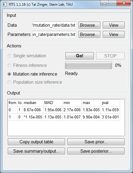
Mutation rate inference

A common problem is the inference of the rates of mutations between two (or more) alleles. FITS supports such inference by harnessing prior knowledge about the fitness of the mutant allele(s) (say, from competition essay) and and the size of the population. A particular example for a case where such inference can be highly accurate is the usage of frequencies of multiple positions with equal fitness. In many biological entities synonyomus mutations approach neutrality and therefore may be used for mutation rate inference. In this example we’ll highlight how this can be done. We simulated 10 independent loci using fitness value of 1, population size of 100,000 and mutation rate of 10^-5 and measured their frequencies for 15 generations.

The minimum and maximum considerable mutations rates should be provided within the parameters file, using the log value. For this example, we use considerable mutation rates between 10^-7 and 10^-3, which will be defined between the wildtype allele (0) and the mutant allele (1) and vice-versa. For providing the minimal log mutation rate between the wildtype allele and the mutant we set min_log_mutation_rate0_1 -7 and its reciprocal min_log_mutation_rate1_0 -7. For providing the maximal log mutation rate between the wildtype allele and the mutant we set max_log_mutation_rate0_1 -3 and its reciprocal max_log_mutation_rate1_0 -3.

We used neutral alleles and therefore set the wildtype and mutant alleles’ fitness to be one: fitness_allele0 1.0 and fitness_allele1 1.0.

The data file for simulated neutral alleles (fitness of 1) under a populations size of 10⁵ and a mutation rate of 10^-5 is available here. The corresponding parameters file is available here.

FITS inferred 0 → 1 mutation rate of 8.67*10^-6, and 1 → 0 mutation rate of 1.15*10^-5.

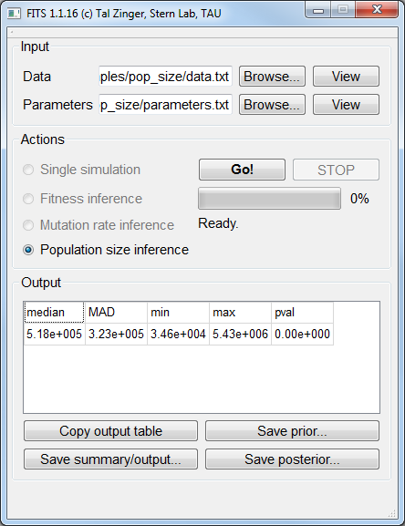
Population size inference

If the mutation rates are known and the fitness of the measured allele is known, then the population size parameter may be inferred. Similar to the mutation rate inference, this can be performed by using frequency data from several loci that has the same fitness values. Here we simulated 10 neutral positions for 15 generations, using a population size of 100,000 and a mutation rate of 10^-5.

Our prior knowledge suggests that the population size may be in the range between 10⁴ and 10⁷. We therefore set the parameter Nlog_min 4 to indicate minimum population size of 10⁴. We also set the parameter Nlog_max 7 to indicate the maximum population size of 10⁷.

Our prior knowledge also suggests that the alleles we measured are neutral, and therefore we set the wildtype and mutant alleles to have a fitness of 1: fitness_allele0 1.0 and fitness_allele1 1.0.

Other parameters such as mutation rates, number of simulations and the sampling rate are similar to the Fitness inference example. The example data file is available here. The corresponding parameters file is available here.

FITS inferred a population size of 5.18*10⁵.

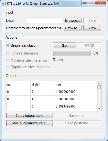
Trajectory simulations

Sometimes, we wish to have frequency data generated. Since simulations are a cornerstone on which FITS is relying on, it is possible to ask the framework to perform simulations of frequencies for given mutation rates, population size and fitness value.

In order to do so, we need to provide these three parameters as described in previous examples. For this example, we’ll use a mutation rate of 10^-3, a fitness of 1.02 and a population size of 10⁵.

We wish to simulate two alleles only. We therefore set num_alleles 2 to indicate two alleles.

We set for the two alleles the fitness values of 1 for the wildtype and 1.02 for the mutant: fitness_allele0 1.0 and fitness_allele1 1.02.

We set the corresponding (equal) mutation rates: mutation_rate0_1 0.001 and mutation_rate1_0 0.001.

The population size is set by defining N 100000.

The last two things to consider are the frequency of the alleles in the beginning of the simulation, and the number of generations to simulate. Here we will assume that the wildtype allele is fixated for the beginning of the simulation. We’ll therefore set init_freq_allele0 1 and init_freq_allele1 0. To control for the number of generations (100 in our example) we set num_generations 100.

Note

There’s no need to load a Data file in order to perform the simulations.

Simulation results are available in the Output area.

Considering Sample Effect

Population bottlenecks are common during any evolutionary scenario, whether in vivo or in vitro in experimental populations. In particular during serial passaging, only a fraction of the progeny will be carried on to the next passage. An additional layer of sampling also exists: the number of genomes that are sampled to be sequenced may often be much smaller than the population size itself. FITS can account for both of these types of sampling effects by using the following three parameters: bottleneck_size, bottleneck_interval and sample_size , as illustrated below: